grid attribute object defines a transform $U$ to diagonalize the permittivity. $U$ is often a simple rotation matrix.
in the material database, create a diagonal anisotropic material
on the material tab of a structure object,
select the defined diagonal anisotropic material
link the LC grid attribute to the object( grid attribute property)
LC rotation
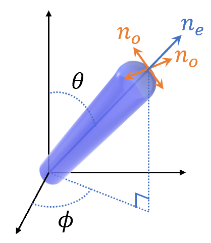
The Liquid crystal (LC) rotation grid attribute allows you to specify a spatially varying LC director orientation in terms of $\theta$, $\phi$.
LC director orientation
Liquid crystals are composed of rod-like molecular structures which have rotational symmetry with respect to a long axis. Therefore, liquid crystals have spatially varying uni-axial optical properties. The refractive indices with respect to the long and short molecular axes are called extraordinary $n_e$ and ordinary $n_o$ respectively, see figure above.
Rotational symmetry allows the transformation matrix to reduced to a function of two rotational angles ($\theta$, $\phi$).
KaTex Tip
\begin{aligned} can’t be on its own line. Nor can \end{aligned}.
You need to use four \s instead of two because they need to be escaped.
You must have a trailing space at the end of those four \s.
and the permittivity tensor in the reference (or simulation ) coordinate system $(x,y,z)$ is transformed to the principal coordinate system $(X,Y,Z)$ via a rotation about $z$, and the $y$.
we have the transform relation:
$$\begin{bmatrix} X\\ Y\\ Z \end{bmatrix} = U(\theta, \phi) \begin{bmatrix} x\\ y\\ z \end{bmatrix} $$
is the permittivity in the principle coordinate system $(X,Y,Z)$.
Uniform distribution
It is quite simple.
In LC attribute object, set the properties “theta” and ‘phi".
Spatially varying orientation distribution of LCs
Importing data using the script environment
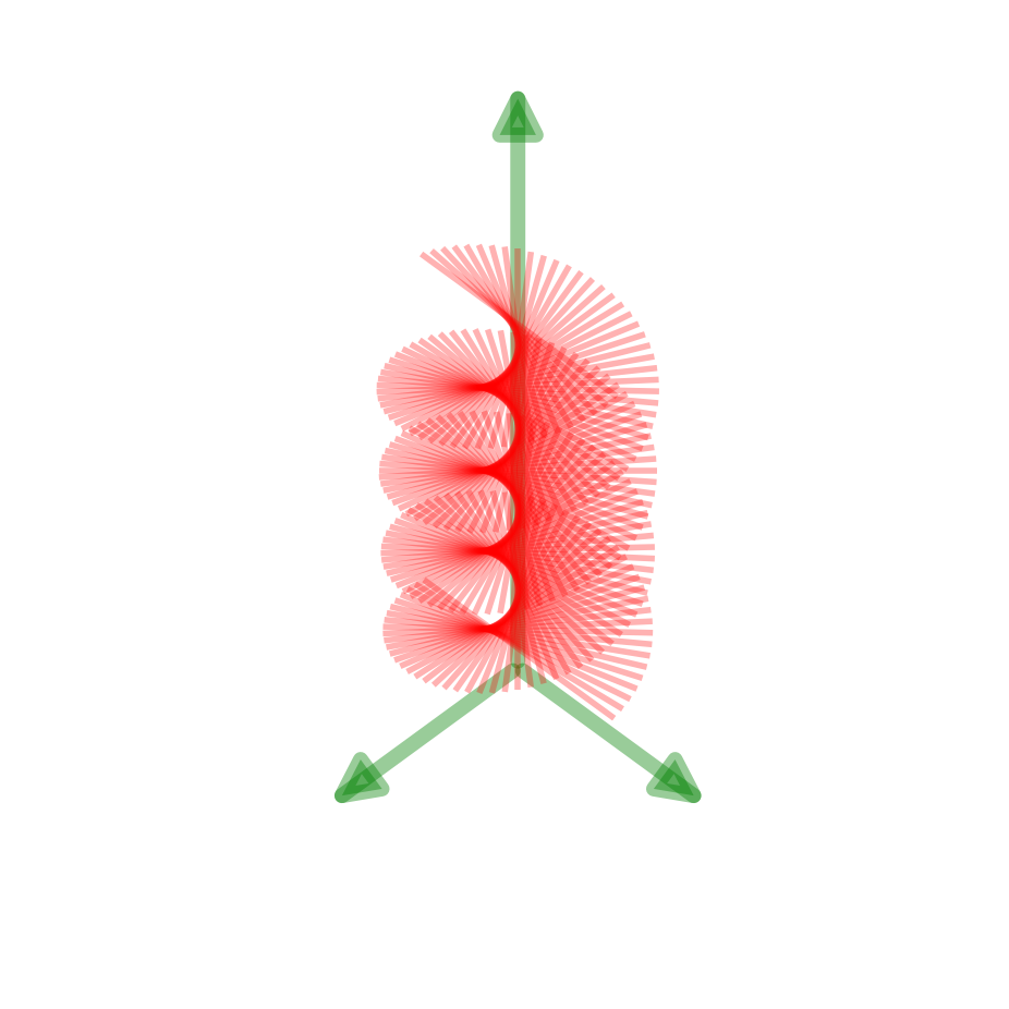
In this case, we can use the addgridattribute , and optionally the importdataset script command to add the LC attribute and to set the spatially varying LC orientation. For example, if we want to set up LCs which are twisted in z direction as shown below, where the components of the LC director are given by
# %matplotlib widget# %matplotlib widget%matplotlibinline%configInlineBackend.figure_format='svg'# %config InlineBackend.figure_format = 'retina'importmatplotlib.pyplotaspltfrommpl_toolkits.mplot3d.proj3dimportproj_transformfrommpl_toolkits.mplot3d.axes3dimportAxes3Dimportnumpyasnpfrommatplotlib.patchesimportFancyArrowPatchclassArrow3D(FancyArrowPatch):def__init__(self,x,y,z,dx,dy,dz,*args,**kwargs):super().__init__((0,0),(0,0),*args,**kwargs)self._xyz=(x,y,z)self._dxdydz=(dx,dy,dz)defdraw(self,renderer):x1,y1,z1=self._xyzdx,dy,dz=self._dxdydzx2,y2,z2=(x1+dx,y1+dy,z1+dz)xs,ys,zs=proj_transform((x1,x2),(y1,y2),(z1,z2),self.axes.M)self.set_positions((xs[0],ys[0]),(xs[1],ys[1]))super().draw(renderer)def_arrow3D(ax,x,y,z,dx,dy,dz,*args,**kwargs):'''Add an 3d arrow to an `Axes3D` instance.'''arrow=Arrow3D(x,y,z,dx,dy,dz,*args,**kwargs)ax.add_artist(arrow)setattr(Axes3D,'arrow3D',_arrow3D)defLC_twist_z_axis():withplt.style.context(['science','notebook']):fig=plt.figure(dpi=100)ax=plt.axes(projection='3d')# Make the gridx,y,z=np.meshgrid(0,0,np.arange(0,4,0.03))# Make the direction data for the arrowsux=np.cos(np.pi*z)uy=np.sin(np.pi*z)uz=np.zeros(z.shape)ax.quiver(x,y,z,ux,uy,uz,length=0.05,arrow_length_ratio=0,pivot='middle',normalize=True,colors='red',alpha=0.3,linestyles='solid')ax.arrow3D(0,0,-0.25,0,-0.05,0,mutation_scale=30,arrowstyle="-|>",linestyle='solid',color='green',alpha=0.4,linewidth=5)ax.arrow3D(0,0,-0.25,0.05,0,0,mutation_scale=30,arrowstyle="-|>",linestyle='solid',color='green',alpha=0.4,linewidth=5)ax.arrow3D(0,0,-0.25,0,0,7,mutation_scale=30,arrowstyle="-|>",linestyle='solid',color='green',alpha=0.4,linewidth=5)ax.grid(False)ax.axis(False)ax.view_init(elev=45,azim=-45)plt.show()LC_twist_z_axis()
LC directors twisted along z-axis
we define the director distribution in a matrix variable and put the matrix into the LC attribute property. In the following script, matrix “n” is used to define the director distribution of the twisted nematic LCs, and this information is put into a dataset called LC which contains the x, y, z position data and the director orientations in an attribute called “u”. At the second last line where addgridattribute command is used, a LC attribute is added to the simulation and the director distribution is set up.
Note : Magnitude of spatially varying orientation unit vector
When specifying the LC orientation, it is important that the magnitude of the orientation vector be exactly 1, except in regions where you don’t want the LC orientation to be set where the magnitude of the vector should be set to 0.
# define x/y/z
x = 0;
y = 0;
z = linspace(0e-6,5e-6,100);
X = meshgrid3dx(x,y,z);
Y = meshgrid3dy(x,y,z);
Z = meshgrid3dz(x,y,z);
n = matrix(length(x),length(y),length(z),3);

# define the orientation function
n(1:length(x),1:length(y),1:length(z),1) = cos(Z*pi*1e5);
n(1:length(x),1:length(y),1:length(z),2) = sin(Z*pi*1e5);
n(1:length(x),1:length(y),1:length(z),3) = 0;

# create dataset containing orientation vectors and position parameters
LC=rectilineardataset("LC",x,y,z);
LC.addattribute("u",n);

# add LC import grid attribute
addgridattribute("lc orientation",LC);
setnamed("LC attribute","nz",50); # set resolution
Note : When setting angle theta via ‘set’ script command, the input must be in radians. For example:
1
setnamed("LC attribute","theta",pi/4);
We then add a material with diagonal anisotropy components and set up the object to use the LC attribute similarly to the case of uniform distribution.
importimportlibfromcollectionsimportOrderedDictfromscipyimportinterpolateimportmatplotlib.pyplotaspltimportmatplotlib.cmascmfromscipyimportconstantsfromnumpy.lib.scimathimportsqrt# complex sqrt()importnumpyasnp%matplotlibinline# import mplcursors # for data cursor# import sys# The default paths for windowsspec=importlib.util.spec_from_file_location('lumapi','D:\\Program Files\\Lumerical\\v202\\api\\python\\lumapi.py')# Functions that perform the actual loadinglumapi=importlib.util.module_from_spec(spec)spec.loader.exec_module(lumapi)fdtd=lumapi.FDTD()# an empty instance# define x/y/zx=0y=0z=np.linspace(0e-6,5e-6,100)X,Y,Z=np.meshgrid(x,y,z)# define n# n = np.zeros((x.size,y.size,z.size,3));nx=np.cos(np.pi*Z*1e5)ny=np.sin(np.pi*Z*1e5)nz=np.zeros(Z.shape)# The newaxis object can be used in all slicing operations to# create an axis of length one. np.newaxis is an alias for ‘None’n=np.concatenate((nx[...,np.newaxis],ny[...,None],nz[...,None]),axis=3)# create dataset containing orientation vectors and position parametersLC=fdtd.rectilineardataset("LC",x,y,z)lumapi.addattribute(LC,'u',n)# add LC import grid attributefdtd.addgridattribute("lc orientation",LC)fdtd.set('name','LC_attribute')fdtd.setnamed("LC_attribute","nz",50)# set resolution
Importing data from .mat file using the graphical user interface
In the edit window of the grid attribute, it is possible to import a .mat file containing a dataset with the required director distribution data by clicking on the “Import data…” button. The following code shows an example of how to save a .mat file to be imported by using the matlabsave script command.
# define x/y/z
x = 0;
y = 0;
z = linspace(0e-6,5e-6,100);
X = meshgrid3dx(x,y,z);
Y = meshgrid3dy(x,y,z);
Z = meshgrid3dz(x,y,z);
n = matrix(length(x),length(y),length(z),3);

# define the orientation function
n(1:length(x),1:length(y),1:length(z),1) = cos(Z*pi*1e5);
n(1:length(x),1:length(y),1:length(z),2) = sin(Z*pi*1e5);
n(1:length(x),1:length(y),1:length(z),3) = 0;

# create dataset containing orientation vectors and position parameters
LC=rectilineardataset("LC",x,y,z);
LC.addattribute("u",n);

# save data to .mat file
matlabsave("LC_import.mat",LC);
We then add a material with diagonal anisotropy components and set up the object to use the LC attribute similarly to the case of uniform distribution.
Importing data from a CSV (comma-separated values) file
From the Import menu in the top toolbar, click on Import from CSV to open the import wizard which allows you to select the CSV file to import. This file is typically created with TechWiz LCD from Sanayi System Co., Ltd (http://sanayisystem.com/).
For more details on the file format and steps for importing the data from the graphical wizard, see Import object - Liquid crystal from CSV.
The same data can also be imported using the importcsvlc script command.